There are many uses for the sentiment of tweets a company is receiving, a few examples are:
- You are attempting to create a poll for a party that is running for government and want to see the sentiment of the people on Twitter, of which we can plot the results by the location the tweet came from. Using these results you could choose to target your marketing to boost numbers in the regions of low sentiment.
- You wish to track a certain individual or multiple individuals to ascertain their thoughts on topics, for example the CEO’s of the top 500 companies. From the results you may choose to invest in certain commodities.
- You are running a marketing campaign and are interested in how the active Twitter population feels about your advertisements.
In this project I have explored the use of the Twitter streaming API in R as a means to gather data throughout the period of a day. I then attempted to create some sentimental inferences about the tweets. I’ve tried to walk through some of the code for those who aren’t familiar with R or programming in general.
Required packages and data
To get the data I used for this project download all files from my public dropbox folder: Supermarket Dropbox
1
2
3
4
5
6
|
#Set working directory
setwd("/Users/andrewchallis/Desktop/R-projects/Sentiment Analysis/Supermarkets/")
#Installing all the packages efficently
x<-c("streamR","RCurl", "RJSONIO", "stringr","ROAuth", "ggplot2", "ggthemes", "Amelia", "plyr")
lapply(x,install.packages(x),character.only=T)
lapply(x,library,character.only=T)
|
Setting up a Twitter handshake
Firstly we need to authenticate ourselves to Twitter - this is done by a ‘handshake’ just how you introduce yourself in an interview. This is done by firstly creating a Twitter account, then going to apps.twitter.com -> ‘My apps’ -> ‘Create new app’ and filling in the details. If you don’t have a website you can use a placeholder. For example I used the placeholder: test.de/
The key information we need from the next page is the ‘Consumer Key (API Key)’ and the ‘Consumer Secret (API Secret)’. We will store these as variables in R note the keys I display are examples and not my keys. Now we can add our variables into R, insert your keys as required.
 1
 2
 3
 4
 5
 6
 7
 8
 9
10
11
12
13
14
|
# PART 1: Declare Twitter API Credentials & Create Handshake
requestURL <- "https://api.twitter.com/oauth/request_token"
accessURL <- "https://api.twitter.com/oauth/access_token"
authURL <- "https://api.twitter.com/oauth/authorize"
consumerKey <- "OaRKbsmfkmhptUv67hfcHwcBnrK" # From dev.twitter.com
consumerSecret <- "Pj45Hqrd1f1Dn0FfqgayPjVgQIdUgkevyPDn3F621aqeT" # From dev.twitter.com

my_oauth <- OAuthFactory$new(consumerKey = consumerKey,
                             consumerSecret = consumerSecret,
                             requestURL = requestURL,
                             accessURL = accessURL,
                             authURL = authURL)

my_oauth$handshake(cainfo = system.file("CurlSSL", "cacert.pem", package = "RCurl"))
|
After you have successfully run the previous code (and only after!) then we can then save this authorisation certificate and get to the good stuff! To save this simply run:
1
2
|
# PART 2: Save the my_oauth data to an .Rdata file
save(my_oauth, file = "my_oauth.Rdata")
|
Let’s get the data!
Now we are ready to search Twitter. I am going to look for tweets that mention any of the UK’s top 5 supermarkets. To do this I look for @asda, @sainsburys, @Tesco, @Morrisons and @AldiUK. If you want to try something else then simply change the vector! For example, if you searched “to:BarackObama” then we would get a live feed of tweets that people are sending to Obama’s Twitter page.
This code will track the tags we give it, only return tweets in english the english language. It will also be persistent so won’t timeout and will save the tweets to the filename tweets.json. Note that the tweets will always be appended, so if you try searching for a different term then you should either delete your old json file or change the file name.
1
2
3
4
5
6
7
|
load("my_oauth.Rdata")

filterStream(file.name = "tweets.json", # Save tweets in a json file
             track = c("@asda", "@sainsburys", "@Tesco", "@Morrisons", "@AldiUK"),
             language = "en",
             timeout = 0, # Keep connection alive persistently (change to 10 for 10 seconds, 60 for 60 seconds etc)
             oauth = my_oauth) # Use my_oauth file as the OAuth credentials
|
Now we can parse the json file and bring it into R as a dataframe.
1
|
temp <- parseTweets("Data/tweets.json", simplify = FALSE) # parse the json file and save to a data frame called tweets.df. Simplify = FALSE ensures that we include lat/lon information in that data frame.
|
Now let’s make use of a great library called Amelia which looks at the missingness of data - This library was named after American Aviation pioneer and author Amelia Earhart, who was the first female aviator to fly solo across Atlantic Ocean in 1932. However, she vanished while trying to establish a record as the first woman to fly around the world on July 2, 1937. No proof was found whether she is alive/dead.
1
2
3
4
|
missmap(temp, col = c("#FF6961", "#222222"), legend = FALSE,
               main = "Missing values from Supermarket Twitter corpus",
               y.labels = c(""),
               y.at = c(1))
|
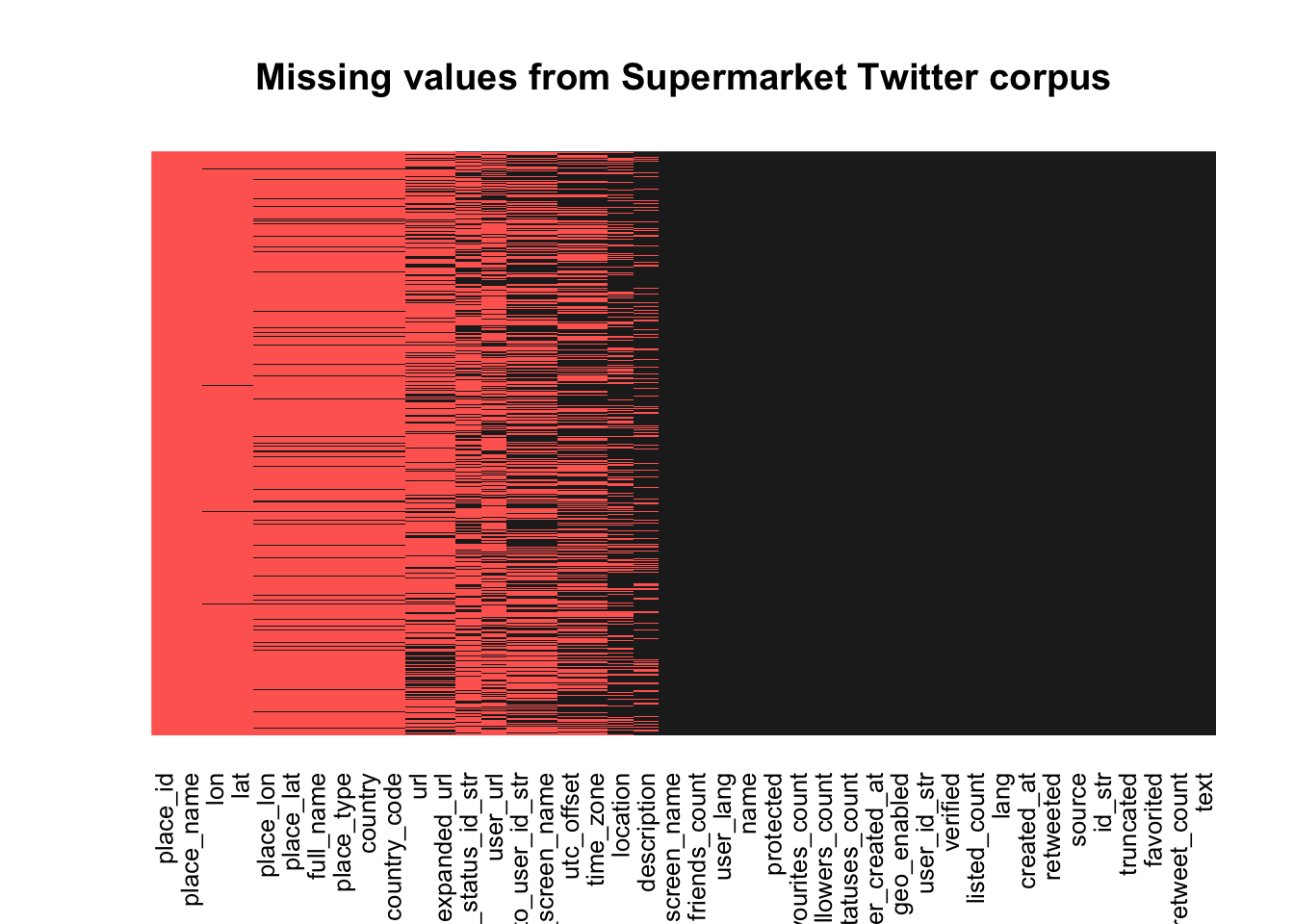
Notice that there are a lot of useless columns in our data frame, so let’s remove the ones we don’t want by setting them to NULL. Let’s also remove any of the columns that have too much missing data to be useful.
1
2
3
4
5
6
7
|
# Don't want any of these:
unwanted.columns = c("url", "place_id", "place_id", "place_name", "lat", "lon", "place_lon", "place_lat",
"full_name", "place_type", "country_code", "in_reply_to_status_id_str", "in_reply_to_screen_name",
"in_reply_to_user_id_str", "lang", "expanded_url", "time_zone", "utc_offset", "user_url", "geo_enabled", "country")

# Let's remove them all from the temp dataframe
temp = temp[ , !(names(temp) %in% unwanted.columns)]
|
Now we have removed all of the data we felt was useless (or too much of it was missing to be useful). Let’s look at our new missingness map.
1
2
3
4
|
missmap(temp, col = c("#FF6961", "#222222"), legend = FALSE,
               main = "Missing values from Supermarket Twitter corpus",
               y.labels = c(""),
               y.at = c(1))
|
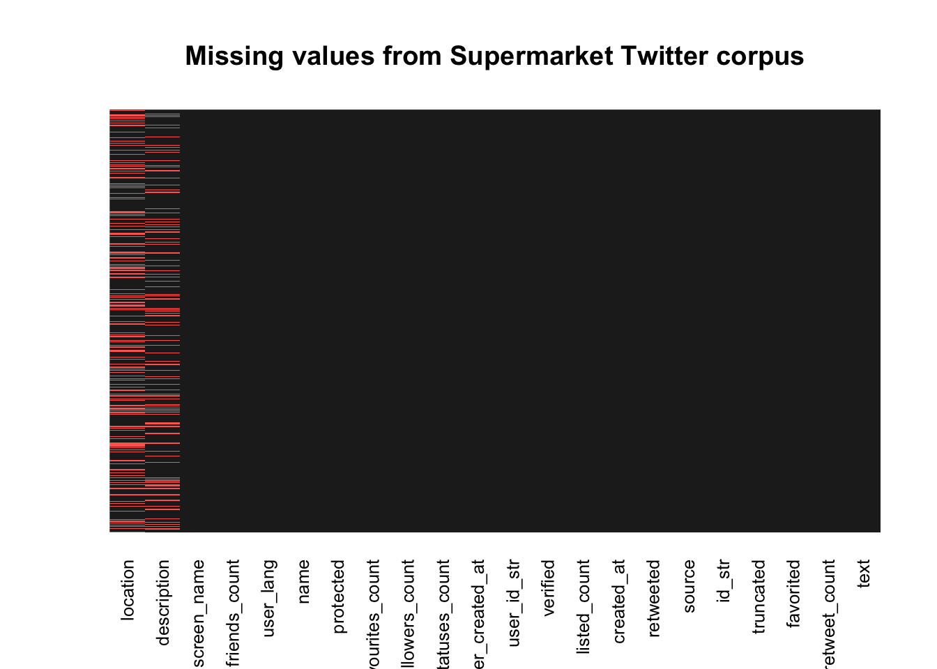
This looks better! Notice that the missing data left is just: The location and profile description of the user as defined in their account settings (not location of the tweet).
Next we should check the structure of the data frame.
 1
 2
 3
 4
 5
 6
 7
 8
 9
10
11
12
13
14
15
16
17
18
19
20
21
22
23
|
## 'data.frame':    8662 obs. of  22 variables:
##  $ text            : chr  "@sainsburys Ha, no apology needed, just checking both worked before handing one over - hope nobody is in trouble at your end! ;"| __truncated__ "@sainsburys yeah every time i go there they don't have it" "@Morrisons no I don't sorry. I would suggest making sure the out of date ones are removed from the shelf,also answe… https://t."| __truncated__ ".@Tesco Apologies in advance for the impact this will have on your Napoleon brandy-related profits." ...
##  $ retweet_count   : num  0 0 0 0 0 1 0 0 0 1 ...
##  $ favorited       : logi  FALSE FALSE FALSE FALSE FALSE FALSE ...
##  $ truncated       : logi  FALSE FALSE TRUE FALSE FALSE FALSE ...
##  $ id_str          : chr  "806870536588578816" "806870550584971265" "806870582688120832" "806870714267660288" ...
##  $ source          : chr  "<a href=\"https://twitter.com\" rel=\"nofollow\">Twitter Web Client</a>" "<a href=\"https://twitter.com/download/android\" rel=\"nofollow\">Twitter for Android</a>" "<a href=\"https://twitter.com/download/android\" rel=\"nofollow\">Twitter for Android</a>" "<a href=\"https://twitter.com\" rel=\"nofollow\">Twitter Web Client</a>" ...
##  $ retweeted       : logi  FALSE FALSE FALSE FALSE FALSE FALSE ...
##  $ created_at      : chr  "Thu Dec 08 14:38:21 +0000 2016" "Thu Dec 08 14:38:24 +0000 2016" "Thu Dec 08 14:38:32 +0000 2016" "Thu Dec 08 14:39:03 +0000 2016" ...
##  $ listed_count    : num  25 6 0 7 12 113 614 31 7 119 ...
##  $ verified        : logi  FALSE FALSE FALSE FALSE FALSE FALSE ...
##  $ location        : chr  "Yorkshire" "Berkshire England" "Aberdeen" "Thurso, Scotland" ...
##  $ user_id_str     : chr  "229868395" "22800342" "69847794" "37244651" ...
##  $ description     : chr  "Kathryn has been something of an enigma this year. - my fifth year Maths teacher." "Love my Rescue Jack Russell Molly soooo much! Shes my baby! &  Music is life. #drizzy #yolo. Dogs r gods" NA "PhD researcher - marine plastics and emerging pollutants. I like tea, wild naps, and cycling. Opinions are mine, obviously." ...
##  $ user_created_at : chr  "Thu Dec 23 15:11:40 +0000 2010" "Wed Mar 04 17:06:16 +0000 2009" "Sat Aug 29 11:34:08 +0000 2009" "Sat May 02 17:49:10 +0000 2009" ...
##  $ statuses_count  : num  3314 2041 2264 11339 5058 ...
##  $ followers_count : num  649 458 330 476 432 ...
##  $ favourites_count: num  302 2502 259 2929 3437 ...
##  $ protected       : logi  FALSE FALSE FALSE FALSE FALSE FALSE ...
##  $ name            : chr  "Kat" "Laura Marie Allen" "Jenna Allan" "Emily Kearl" ...
##  $ user_lang       : chr  "en" "en" "en" "en" ...
##  $ friends_count   : num  2104 2133 821 599 178 ...
##  $ screen_name     : chr  "LeChatMystique" "Lauskissbabe" "xxjennatronxx" "emilykearl" ...
|
There are a few of these columns with odd data structures such as ‘created_at’ which should be a date-time not a character! Similarly ‘user_created_at’ should be a date-time. Run the following code to change these.
# Changing date format to Posixct
temp$created_at = strptime(temp$created_at, format = "%a %b %d %H:%M:%S %z %Y")
temp$created_at = as.POSIXct(temp$created_at)
temp$user_created_at = strptime(temp$user_created_at, format = "%a %b %d %H:%M:%S %z %Y")
temp$user_created_at = as.POSIXct(temp$user_created_at)
A lot of the tweets contain emojis which are in UTF-8 encoded text. To make things easier we will remove these emojis. (This is part of my second project to incorporate emojis as part of the sentiment analysis so look out for it!).
The code below will remove any graphical parameters from the tweet (text), the username the tweet belongs to and their profile description.
1
2
3
|
temp$text=str_replace_all(temp$text,"[^[:graph:]]", " ")
temp$name=str_replace_all(temp$name,"[^[:graph:]]", " ")
temp$description=str_replace_all(temp$description,"[^[:graph:]]", " ")
|
Let’s have a final check of the structure of the data frame.
 1
 2
 3
 4
 5
 6
 7
 8
 9
10
11
12
13
14
15
16
17
18
19
20
21
22
23
|
## 'data.frame':    8662 obs. of  22 variables:
##  $ text            : chr  "@sainsburys Ha, no apology needed, just checking both worked before handing one over - hope nobody is in trouble at your end! ;"| __truncated__ "@sainsburys yeah every time i go there they don't have it" "@Morrisons no I don't sorry. I would suggest making sure the out of date ones are removed from the shelf,also answe… https://t."| __truncated__ ".@Tesco Apologies in advance for the impact this will have on your Napoleon brandy-related profits." ...
##  $ retweet_count   : num  0 0 0 0 0 1 0 0 0 1 ...
##  $ favorited       : logi  FALSE FALSE FALSE FALSE FALSE FALSE ...
##  $ truncated       : logi  FALSE FALSE TRUE FALSE FALSE FALSE ...
##  $ id_str          : chr  "806870536588578816" "806870550584971265" "806870582688120832" "806870714267660288" ...
##  $ source          : chr  "<a href=\"https://twitter.com\" rel=\"nofollow\">Twitter Web Client</a>" "<a href=\"https://twitter.com/download/android\" rel=\"nofollow\">Twitter for Android</a>" "<a href=\"https://twitter.com/download/android\" rel=\"nofollow\">Twitter for Android</a>" "<a href=\"https://twitter.com\" rel=\"nofollow\">Twitter Web Client</a>" ...
##  $ retweeted       : logi  FALSE FALSE FALSE FALSE FALSE FALSE ...
##  $ created_at      : POSIXct, format: "2016-12-08 14:38:21" "2016-12-08 14:38:24" ...
##  $ listed_count    : num  25 6 0 7 12 113 614 31 7 119 ...
##  $ verified        : logi  FALSE FALSE FALSE FALSE FALSE FALSE ...
##  $ location        : chr  "Yorkshire" "Berkshire England" "Aberdeen" "Thurso, Scotland" ...
##  $ user_id_str     : chr  "229868395" "22800342" "69847794" "37244651" ...
##  $ description     : chr  "Kathryn has been something of an enigma this year. - my fifth year Maths teacher." "Love my Rescue Jack Russell Molly soooo much! Shes my baby! &  Music is life. #drizzy #yolo. Dogs r gods" NA "PhD researcher - marine plastics and emerging pollutants. I like tea, wild naps, and cycling. Opinions are mine, obviously." ...
##  $ user_created_at : POSIXct, format: "2010-12-23 15:11:40" "2009-03-04 17:06:16" ...
##  $ statuses_count  : num  3314 2041 2264 11339 5058 ...
##  $ followers_count : num  649 458 330 476 432 ...
##  $ favourites_count: num  302 2502 259 2929 3437 ...
##  $ protected       : logi  FALSE FALSE FALSE FALSE FALSE FALSE ...
##  $ name            : chr  "Kat" "Laura Marie Allen" "Jenna Allan" "Emily Kearl" ...
##  $ user_lang       : chr  "en" "en" "en" "en" ...
##  $ friends_count   : num  2104 2133 821 599 178 ...
##  $ screen_name     : chr  "LeChatMystique" "Lauskissbabe" "xxjennatronxx" "emilykearl" ...
|
Looks good and clean! Now we will move on to some feature engineering where we will find out what device the tweet came from. We’ll also assign categories for each of the tweets depending on which company the tweet was regarding.
Feature engineering
If we look at the head (top of the data frame) of temp$source we can see that this has information about the device the tweet originated from.
1
2
3
4
5
6
|
## [1] "<a href=\"https://twitter.com\" rel=\"nofollow\">Twitter Web Client</a>"
## [2] "<a href=\"https://twitter.com/download/android\" rel=\"nofollow\">Twitter for Android</a>"
## [3] "<a href=\"https://twitter.com/download/android\" rel=\"nofollow\">Twitter for Android</a>"
## [4] "<a href=\"https://twitter.com\" rel=\"nofollow\">Twitter Web Client</a>"
## [5] "<a href=\"https://twitter.com/download/android\" rel=\"nofollow\">Twitter for Android</a>"
## [6] "<a href=\"https://twitter.com/download/android\" rel=\"nofollow\">Twitter for Android</a>"
|
Let’s take out the keywords from these such as ‘ipad’, ‘iphone’ and set them as another column called ‘devices’ in our dataframe. Lets also give the column a data structure of a factor. See below for a description of what the for loop is doing.
First we have to make an empty vector to put the values in which we have called ‘source’. Then for all the rows in our dataframe ‘temp’ do the following:
If there is the pattern ‘android’, then put the ith value of source equal to ‘android’, if not then continue. If there is the pattern ‘iphone’, then put the ith value of source equal to ‘iphone’, if not then continue … (and so on for Web client, ipad, Twitter for windows) … Then if it is none of these then define it as ‘Other’. After all the rows have done this the for loop ends. We then add a new column to temp called ‘devices’ and it is equal to the vector we just created.
 1
 2
 3
 4
 5
 6
 7
 8
 9
10
11
12
13
14
15
16
17
|
source = c()
for (i in 1: nrow(temp)){
  if (grepl("android", temp$source[i])){
    source[i] = "Android"
  }else if (grepl("iphone", temp$source[i])){
    source[i] = "iphone"
  }else if (grepl("Twitter Web Client", temp$source[i])){
    source[i] = "Web Client"
  }else if (grepl("ipad", temp$source[i])){
    source[i] = "ipad"
  }else if (grepl("Twitter for Windows", temp$source[i])){
    source[i] = "Windows"
  }else{
    source[i] = "Other"
  }
}
temp$devices = source
|
Using the same logic we can get the company the tweet was about.
 1
 2
 3
 4
 5
 6
 7
 8
 9
10
11
12
13
14
15
16
17
18
19
20
21
|
company = c()
for (i in 1:nrow(temp)){
  if (grepl("@asda", tolower(temp$text[i]))){
    company[i] = "Asda"
  }else if (grepl("@sainsburys", tolower(temp$text[i]))){
    company[i] = "Sainsburys"
  }else if (grepl("@morrisons", tolower(temp$text[i]))){
    company[i] = "Morrisons"
  }else if (grepl("@aldi", tolower(temp$text[i]))){
    company[i] = "Aldi"
  }else if (grepl("@tesco", tolower(temp$text[i]))){
    company[i] = "Tesco"
  }else{
    company[i] = "Other"
  }
}
temp$Company = company

#For some reason sometimes we get tweets without any company in so we remove those.
temp = temp[temp$Company != "Other",]
temp$Company = as.factor(temp$Company)
|
I have made a basic function to use here which will just give us a few summary lines about our data. This can be useful if you want to keep checking a live stream of data.
 1
 2
 3
 4
 5
 6
 7
 8
 9
10
11
12
13
14
15
16
|
twitter.summary = function(temp){
  pc = round(as.vector(table(temp$Company))*100/nrow(temp), digits = 1)
  dv = round(as.vector(table(temp$devices))*100/nrow(temp), digits = 1)
  sources.summary = paste("Sources summary: There are",sum(temp$clean.source == "Other"), "undefined sources out of", length(temp$clean.source), "tweets")
  date.summary = paste("Date summary: There tweets range in date from",min(temp$created_at), "till", max(temp$created_at))
  user.summary = paste("User summary:There are tweets from",length(unique(temp$id_str)), "unique users out of", length(temp$id_str), "overall tweets")
  company.summary = paste("Company summary: Aldi: ", pc[1], "%  Asda: ", pc[2], "%  Morrisons: ", pc[3],"%  Sainsburys: ", pc[4], "%  Tesco: ", pc[5], "%", sep = "")
  device.summary = paste("Device summary: Android: ", dv[1], "%  Apple: ", dv[2] + dv[3], "%  Web Client: ", dv[5],"%  Windows: ", dv[6], "%  Other: ", dv[4], "%", sep = "")

  print(date.summary)
  print(user.summary)
  print(device.summary)
  print(company.summary)
}
#Let's see the summary of our data
twitter.summary(temp)
|
1
2
3
4
|
## [1] "Date summary: There tweets range in date from 2016-12-08 14:38:21 till 2016-12-10 13:12:49"
## [1] "User summary:There are tweets from 8338 unique users out of 8340 overall tweets"
## [1] "Device summary: Android: 20.6%  Apple: 48.7%  Web Client: 17.6%  Windows: 1.3%  Other: 11.8%"
## [1] "Company summary: Aldi: 8.7%  Asda: 19.7%  Morrisons: 13.4%  Sainsburys: 19.2%  Tesco: 39%"
|
Sentiment analysis
Now we have finished cleaning and prepping our data. We can try to come up with some metrics to describe the sentiment of the tweets. The technique I have used in this project is just a basic ‘bag of words’ which come from a dictionary of positive and negative words. However, I have also included a phrase dictionary. All of these dictionaries can be edited, so add anything you believe may come up in a tweet. Personally I added ‘out of date’ to the phrase dictionary, these phrases will depend on the type of tweet. For instance no one would tweet with the phrase ‘out of date’ to @Build-A-BearWorkshop.
I also added some bias to the model whereby if any phrase from the dictionary comes up then it would be more negative or positive than just the bag of words dictionary. This is because a user could tweet ‘It’s a good job I checked the sell by date! These green eggs and ham are out of date!’. In the original ‘bag of words’ model the word ‘good’ would have been positive and given a positive sentiment to the tweet (+1 overall). Now with the phrase dictionary included it would still pick up ‘good’ (+1) but it would also pick up ‘out of date’ (-2) so the overall tweet would have a negative sentiment of (-1). This is open to further enhancements, but for this project I just wanted to get a working model.
Lets see the code! First we need to import our dictionaries.
1
2
3
4
|
positives= readLines("Data/positive-words.txt")
negatives = readLines("Data/negative-words.txt")
pos.phrase.list = readLines("Data/pos-phrase-list.txt")
neg.phrase.list = readLines("Data/neg-phrase-list.txt")
|
Now let’s make a function that will take in our dictionaries and a sentence (or vector of sentences) and give us the sentiment of the sentence (or a sentiment vector for all the sentences in the vector).
 1
 2
 3
 4
 5
 6
 7
 8
 9
10
11
12
13
14
15
16
17
18
19
20
21
22
23
24
25
26
27
|
score.sentiment <- function(sentences, pos.words, neg.words, pos.phrase.list, neg.phrase.list, .progress='none'){
  require(plyr)
  require(stringr)
  scores <- laply(sentences, function(sentence, pos.words, neg.words, pos.phrase.list, neg.phrase.list){
    sentence <- gsub('[[:punct:]]', "", sentence)
    sentence <- gsub('[[:cntrl:]]', "", sentence)
    sentence <- tolower(sentence)
    pos.phrase = c()
    for(i in 1:length(pos.phrase.list)){
      pos.phrase[i] = grepl(pos.phrase.list[i], sentence)
    }
    neg.phrase = c()
    for(i in 1:length(neg.phrase.list)){
      neg.phrase[i] = grepl(neg.phrase.list[i], sentence)
    }
    word.list <- str_split(sentence, " ")
    words <- unlist(word.list)
    pos.matches <- match(words, pos.words)
    neg.matches <- match(words, neg.words)
    pos.matches <- !is.na(pos.matches)
    neg.matches <- !is.na(neg.matches)
    score <- sum(pos.matches) - sum(neg.matches) + 2*sum(pos.phrase) - 2*sum(neg.phrase)
    return(score)
  }, pos.words, neg.words, pos.phrase.list, neg.phrase.list, .progress=.progress)
  scores.df <- data.frame(score=scores, text=sentences)
  return(scores.df)
}
|
Now we are finally ready to predict the sentiment of our tweets! Lets pass our dictionaries and temp$text into our newly created function and then add the scores to our dataframe ‘temp’.
1
2
3
4
|
scores.on.the.doors = score.sentiment(temp$text, positives, negatives, pos.phrase.list, neg.phrase.list, .progress='text')

#Add the scores to the data frame
temp$sentiment = scores.on.the.doors$score
|
We haven’t seen a plot in a while so let’s make some!
Pretty visuals
I have edited a ggplot theme here for some nicer visuals. Then set it as the default theme for my plots.
Note I have tried to make the visuals more impacting at the cost of many extra lines of code by assigning the company colors to the graphs so that it is an exact match of asda green or morrisons yellow etc.
 1
 2
 3
 4
 5
 6
 7
 8
 9
10
11
12
13
14
|
myggplot.theme = function (base_size = 12, base_family = "sans") {
  (theme_foundation(base_size = base_size, base_family = base_family) +
     theme(line = element_line(colour = "black"), rect = element_rect(fill = "white", linetype = 0, colour = NA), text = element_text(colour = ggthemes_data$fivethirtyeight["dkgray"]),
           axis.text = element_text(),
           axis.ticks = element_blank(), axis.line = element_blank(),
           legend.background = element_rect(), legend.position = "bottom",
           legend.direction = "horizontal", legend.box = "vertical",
           panel.grid = element_line(colour = NULL), panel.grid.major = element_line(colour = ggthemes_data$fivethirtyeight["medgray"]),
           panel.grid.minor = element_blank(), plot.title = element_text(hjust = 0,
                                                                         size = rel(1.5), face = "bold"), plot.margin = unit(c(1,1, 1, 1), "lines"), strip.background = element_rect()))
}

# Set the theme for all future plots:
theme_set(myggplot.theme())
|
The first plot we will create is of the number of tweets that mention the companies.
 1
 2
 3
 4
 5
 6
 7
 8
 9
10
11
12
13
14
15
16
17
|
# Between hashes is just a hack and slash way to get the bars in order and show the colors
color.df = data.frame(colors = c("#001F78", "#78BE20", "#FEE133", "#F47320", "#F02E25"),
competitors = c("Aldi", "Asda", "Morrisons", "Sainsburys", "Tesco"))
color.df$color = as.factor(color.df$color)
color.df$competitors = as.factor(color.df$competitors)

#Used to get the ranking of the Companies
order.companys = names(sort(table(temp$Company)))

temp$Company = factor(temp$Company, levels = order.companys)
color.df$competitors = factor(color.df$competitors, levels = order.companys)
color.df = arrange(color.df, competitors)

ggplot(temp, aes(Company)) + geom_bar(aes(fill = Company), alpha = 0.8, color = "black") +
  xlab("Company the tweet mentioned") + ylab("Number of Tweets") +
  ggtitle("Number of tweets with company mentioned")  +
  scale_fill_manual(values = as.character(color.df$color))
|
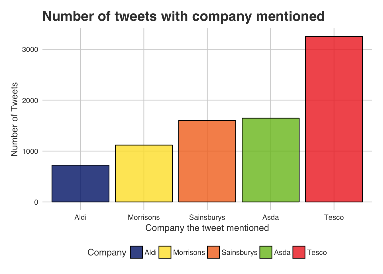
As we can see, currently Tesco seems to have a massive online presence. At Least a lot of mentions, we are yet to see if they carry good or bad sentiments! Also notice that Aldi does not receive many tweets. An interesting thing to look at would be the comparison that these companies spent on online marketing. If anyone could get approximates for this I would love to include it.
Next lets see how many followers people who are tweeting about each company have. This could be interesting, as if people with lots of followers are tweeting about your company then that means they have greater exposure.
1
2
3
4
|
ggplot(temp, aes(factor(Company), followers_count)) + geom_boxplot(aes(color = Company)) +
  xlab("Company") + ylab("Follower count") + ggtitle("Number of followers Twitter users have by the company the tweet was about") +
  coord_cartesian(ylim = c(0,10000)) +
scale_color_manual(values = as.character(color.df$color))
|
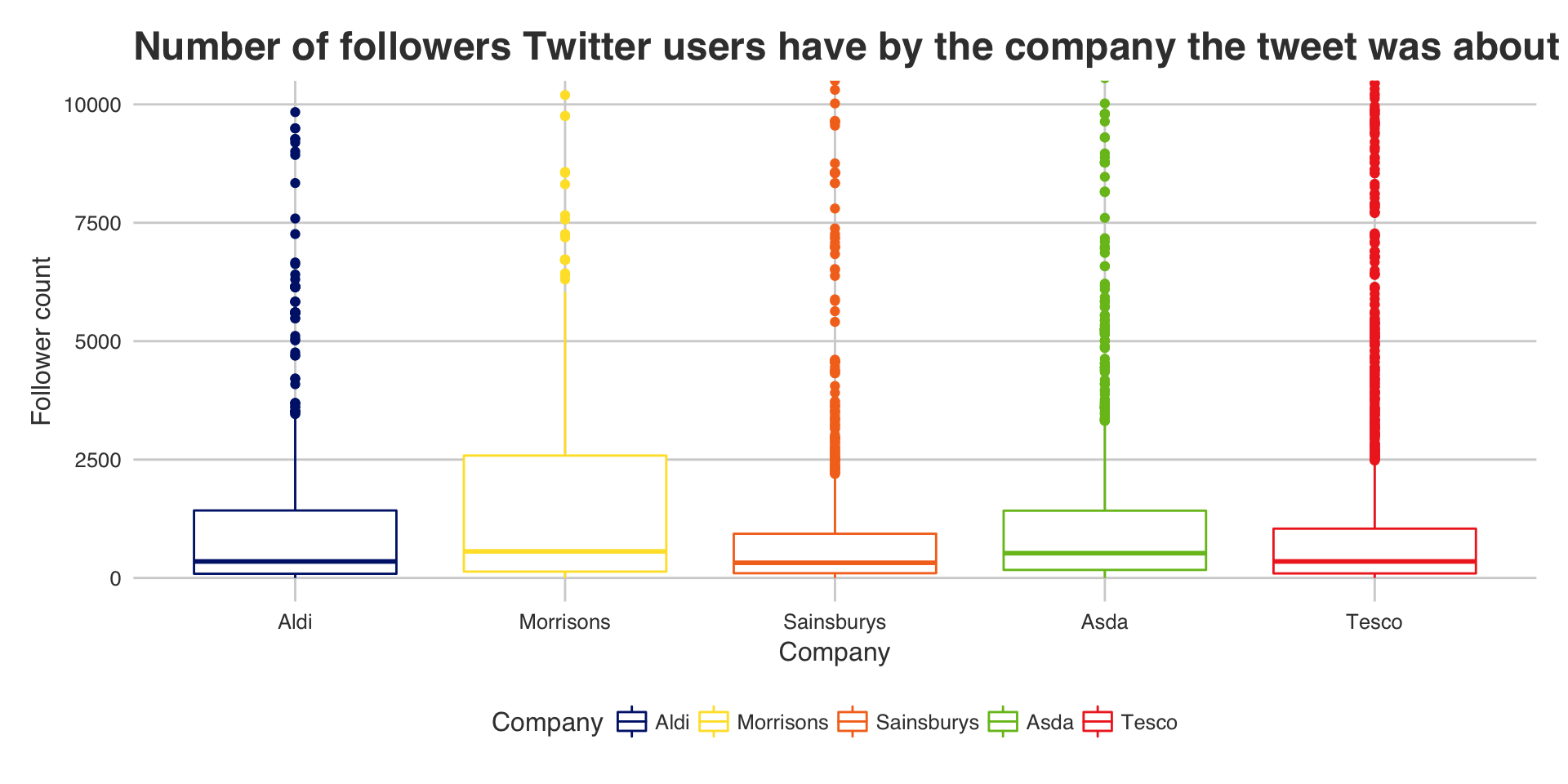
They all seem to have a similar distribution with Sainsburys coming bottom and Morrisons coming top.
Another plot we could make would be the source that the tweets are coming from.
1
2
3
4
5
6
7
8
|
order.devices = names(sort(table(temp$devices)))

temp$devices = factor(temp$devices, levels = order.devices)

ggplot(temp, aes(devices)) + geom_bar(aes(fill = Company), alpha = 0.7, color = "black") +
  xlab("Source of Tweet") + ylab("Number of Tweets") +
  ggtitle("Devices the tweets came from colored by proportion of company") +
scale_fill_manual(values = as.character(color.df$color))
|
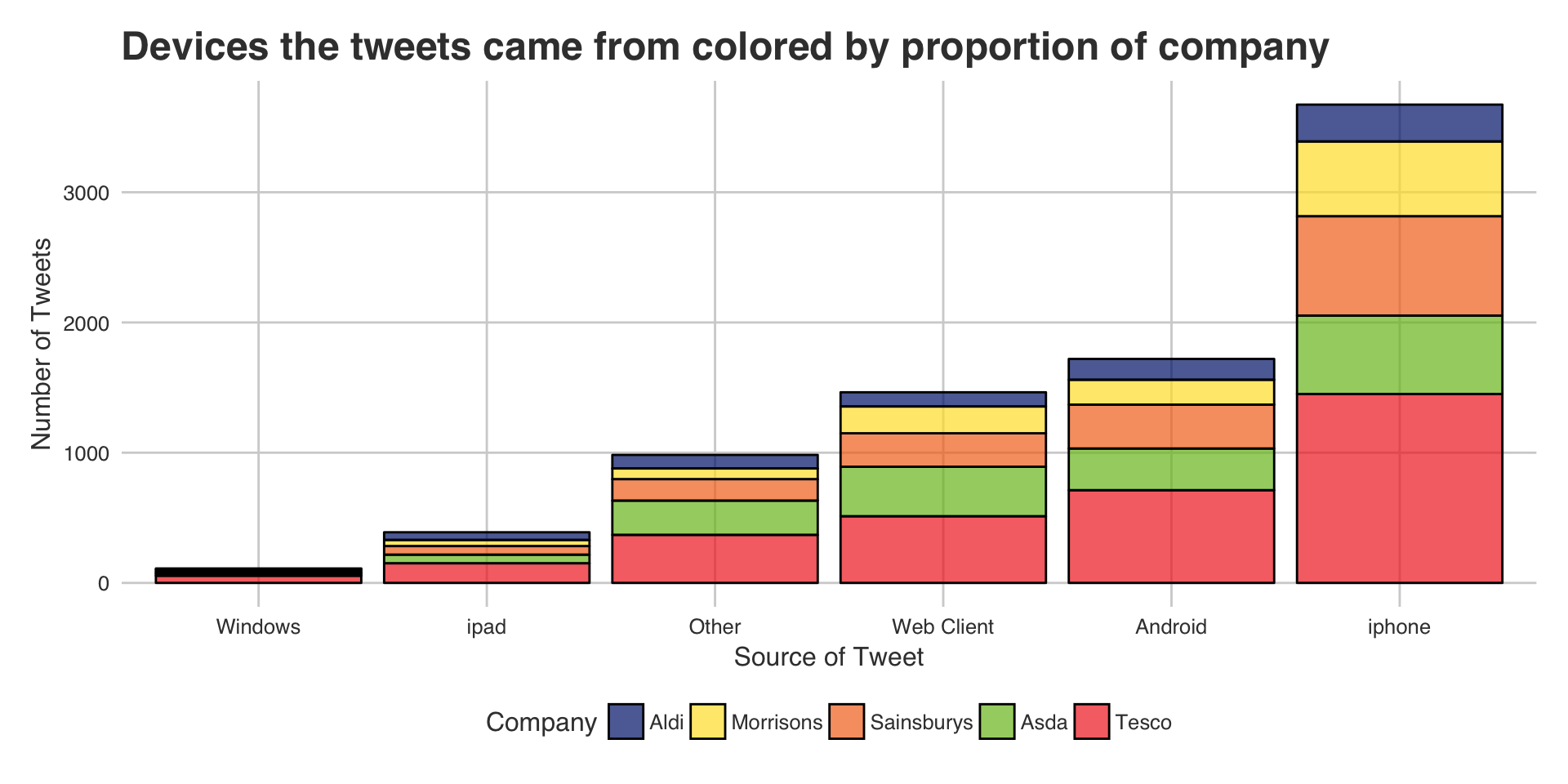
Not surprisingly the majority of the tweets are coming from apple devices. All of the companies seem to have an even distribution of customer devices, This is expected since the companies in question are all very similar. If the companies were instead Iceland and Waitrose, then we could possibly see slightly different distributions There may be more ipads and iphones - since people with a higher disposable income are more likely to shop at waitrose than people with a lower disposable income. (Purely hypothetical)
Now let’s look at the sentiment distributions our ‘bag of words and phrases’ model has given us.
1
2
3
4
5
|
ggplot(temp, aes(sentiment), color = Company) + geom_bar(aes(fill = Company)) +
  facet_grid(Company ~ ., scales = "free") +
  ggtitle("Sentiment score distributions for each company") +
  ylab("# of Tweets") + xlab("Sentiment score") +
  scale_fill_manual(labels=color.df$competitors, values=as.character(color.df$color))
|
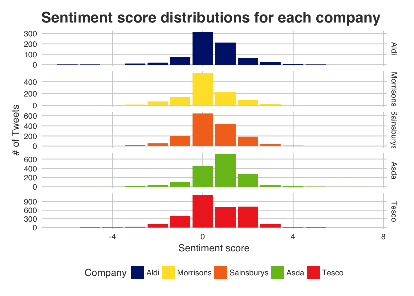
Interestingly Tesco and Asda seem to have the highest sentiment from the tweets, Morrisons seems to be very much neutral whereas Aldi and Sainsburys seem to be equal with slightly positive sentiments.
Similarly we can see if there are any different sentiments by the user’s device. - Maybe everyone with an android device complains but customers with apple devices are happier and send compliments to their favorite supermarket?
1
2
3
|
ggplot(temp, aes(sentiment)) + geom_bar(aes(fill = devices)) +
  facet_grid(devices ~ .) + ggtitle("Sentiment distributions for device used to tweet") +
  ylab("# of Tweets") + xlab("Sentiment score") + scale_fill_discrete(name = "Devices")
|
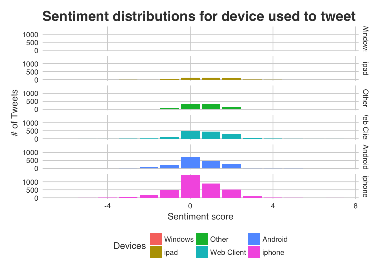
If we look at the ‘web client’, ‘ipad’, ‘windows’ and ‘other devices’ facets they seem to have more of a positively skewed sentiment. ‘iphone’ and ‘android’ are very similar in their sentiment distribution and are only slightly positive. So with this sentiment model and dataset it appears that android users aren’t as willing to give out compliments!
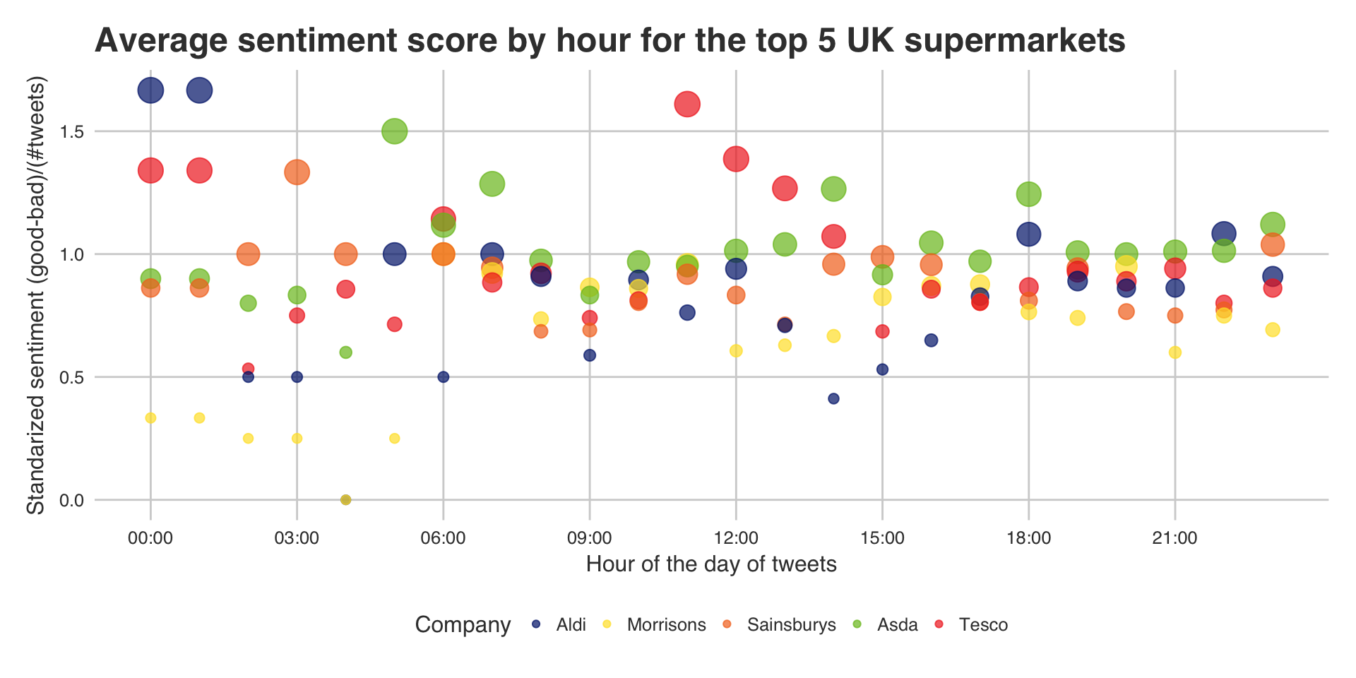
The final plots are trying to be a little fancier. They will display the name of the company by hour (x axis) and the average sentiment for that hour (if they got any tweets). This is a simple calculation of (Positive sentiments in the hour for that company - Negative sentiments in the hour for that company)/(number of tweets that company got that hour). Also the size of the text is proportional to the rank that hour, so the larger the text the better they performed that hour.
 1
 2
 3
 4
 5
 6
 7
 8
 9
10
11
12
13
14
15
16
17
18
19
20
21
22
23
24
25
26
27
28
29
30
31
32
33
34
35
36
37
38
39
40
41
42
43
44
45
46
|
#### RUN THIS FIRST FOR HOUR BY HOUR SENTIMENT PLOT
#############################################################################
ranking = c()
ranking.hour = matrix(nrow = 24, ncol = 5)
hour = as.POSIXlt(temp$created_at)$hour
for(j in 0:23){
  df.hour = temp[hour == j,]
  for (i in 1:length(color.df$competitors)){
    Firm = color.df$competitors[i]
    review = 0
    ranking[i] = sum((df.hour[df.hour$Company==Firm,])[(df.hour[df.hour$Company==Firm,])$sentiment > review,]$sentiment)-
      sum((df.hour[df.hour$Company==Firm,])[(df.hour[df.hour$Company==Firm,])$sentiment < review,]$sentiment)
    if(nrow(df.hour[df.hour$Company==Firm,])>0){
      ranking[i] = ranking[i]/nrow(df.hour[df.hour$Company==Firm,])
    }else{
      ranking[i] = NA
    }
    ranking.hour[j+1,i] = ranking[i]
  }
}

this.hour = rep(0,5)
ranking = ranking.hour[1,]
competitors.rep = rep(color.df$competitors, 24)
color.rep = rep(color.df$color, 24)
for (i in 1:23){
  this.hour = append(this.hour,rep(i,5))
  ranking = append(ranking, ranking.hour[i,])
}

ranking.df = arrange(data.frame(competitors.rep, ranking = ranking, this.hour, color = color.rep), -ranking)
ranking.df = data.frame(ranking.df, rev(seq(1,120, by = 1)))
#ranking.df = arrange(ranking.df, this.hour)
ranking.df$competitors.rep <- factor(ranking.df$competitors.rep, levels = color.df$competitors)
ranking.df$ranking.f = factor(ranking.df$ranking)
#ranking.df[is.na(ranking.df$ranking),]$ranking = 0
#############################################################################

ggplot(ranking.df, aes(x = this.hour, y = ranking, label = competitors.rep)) +
  geom_text(aes(size = ranking.f, color = competitors.rep), alpha = 0.7) +
  scale_color_manual(labels=color.df$competitors, values=as.character(color.df$color)) +
  xlab("Hour of the day of tweets") + ylab("Standarized sentiment (good-bad)/(#tweets)")  +  guides(size=FALSE, color=FALSE)+
  ggtitle("Average sentiment score by hour for the top 5 UK supermarkets") +
  scale_x_continuous(name = "Hour of the day of tweets",
                     breaks = c(0,3,6,9,12,15,18,21),
                     labels = c("00:00", "03:00", "06:00", "09:00", "12:00", "15:00", "18:00", "21:00"))
|
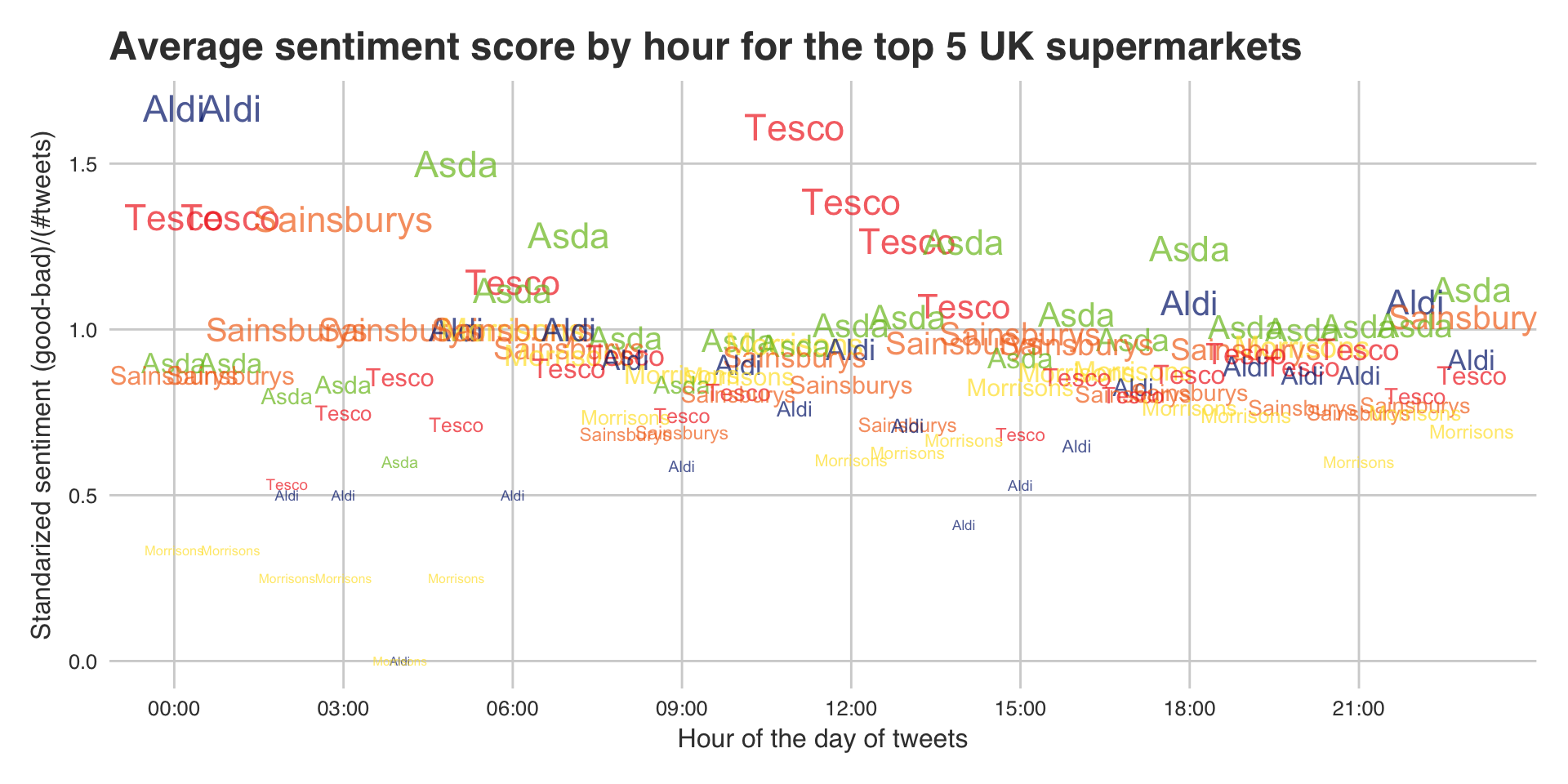
I’m sure there was an easier way to do all that but I was tired while writing it and the hack and slash method worked and wasn’t too slow! If the words are too much and you feel like this is overcrowded then do not fear! I have made another graph that may suit your needs.
1
2
3
4
5
6
7
8
|
ggplot(ranking.df, aes(x = this.hour, y = ranking, label = competitors.rep)) +
  geom_point(aes(size = ranking.f, color = competitors.rep), alpha = 0.7) +
  scale_color_manual(name = "Company",labels=color.df$competitors, values=as.character(color.df$color)) +
  xlab("Hour of the day of tweets") + ylab("Standarized sentiment (good-bad)/(#tweets)")  +  guides(size=FALSE)+
  ggtitle("Average sentiment score by hour for the top 5 UK supermarkets") +
  scale_x_continuous(name = "Hour of the day of tweets",
                     breaks = c(0,3,6,9,12,15,18,21),
                     labels = c("00:00", "03:00", "06:00", "09:00", "12:00", "15:00", "18:00", "21:00"))
|
Next steps
- From here I would like to incorporate some machine learning for the sentiment analysis. My thoughts are to either use a unsupervised learning algorithm such as grouping the text using K-means, or to have some annotated training data with labels of positivity that people believe represent those tweets.
- As mentioned earlier in the document, it would be very advantageous if the model could incorporate emojis into the sentiment. This would be an easy next step to follow on from this since it would only require a positive emoji dictionary and a negative emoji dictionary. Similar to the phrases we may want to weight these depending on how happy or sad the face is.
- More data! Unfortunately I was running this on my laptop and there were a few outages where the Twitter API disconnected, for the next dataset I will run an R script on my home server for around a week. I’d estimate the .json file to be around 250MB which would convert to 30MB .csv after we have removed all of the unwanted data.
- Improving my R coding within this document and refining the graphs - such as the hour by hour, if possible make an interactive graph and the x axis points would be date-time then have a region to select over and display.
- Make code more efficient, I have never had to deal with this before but as the data volumes increase this will be vital.
- As part of my self development I’m going to be coding a similar project up in python at some point. If you have any suggestions for twitter tags or users, locations or keywords to use, let me know and I’ll try to encorporate it.
I would love to have any feedback on this little project so if you have any opinions do let me know! Similarly if you want any help reproducing this or something similar and need any tips do get in contact.
You’ll notice that the json file will get large very fast and it has a lot of columns that we dont want. One quick remedy (though definately not the best) would be as follows:
Run the twitter trawler from your command prompt in the background so it is constantly running - this means you’ll continously gather your data. Then in anther command prompt run the following script. It will take the json file and do all the data manipulation we set out in this tutorial and save the resulting file as a csv. I have set the variables at the top so they can easily be changed.
If you use the code ‘as is’ it will look for the json file ‘example.json’ if it can’t find it then it will wait 30 seconds before trying again. Once it has found the file it will repeatedly wait 5 minutes before trying again until the file is greater than 500000 bytes before it converts it to a csv. If it is the first entry into the csv file it will include the headers, if it isnt then it will just append to the csv. The final csv output will be called ‘Temp.csv’.
(Note this can fail if there was a truncation at speech marks. To fix this I have inculded the lines temp$text = gsub("\"", "", temp$text) and temp$description = gsub("\"", "", temp$description) which will remove “\”" )
(Also note that each time we clear the old json file we have a chance of removing a tweet mid way through proccessing, so the longer the time period between conversion the less tweet loss.)
 1
 2
 3
 4
 5
 6
 7
 8
 9
10
11
12
13
14
15
16
17
18
19
20
21
22
23
24
25
26
27
28
29
30
31
32
33
34
35
36
37
38
39
40
41
42
43
44
45
46
47
48
49
50
51
52
53
54
55
56
57
58
59
60
61
62
63
64
65
66
67
68
69
70
71
72
73
74
75
76
77
78
79
80
81
82
83
84
85
86
87
88
|
directory = "/Users/andrewchallis/Desktop/"
json.file.name = "tweets.json"
csv.file.name = "Temp.csv"
waiting.time = 300
max.json.size = 500000


library(streamR)
options(warn=-1)

while(is.na(file.size(paste(directory, json.file.name, sep = "")))){
  print(paste("There is no json file called '", json.file.name, "' I'll wait 30 seconds and try again", sep = ""))
  Sys.sleep(30)
}
print(paste("I found the json file: '",json.file.name,"' I'll attempt to convert it to a csv...", sep = ""))
if(file.size(paste(directory,json.file.name , sep = ""))>max.json.size){
  print(file.size(paste(directory,json.file.name , sep = "")))
  print("Big file")
  temp = parseTweets(paste(directory,json.file.name , sep = ""), simplify = FALSE)
  #We only want tweets that have text!
  temp = temp[!is.na(temp$text),]

  #Dont want any of these
  unwanted.columns = c("url", "place_id", "place_id", "place_name", "lat", "lon", "place_lon", "place_lat",
                       "full_name", "place_type", "country_code", "in_reply_to_status_id_str", "in_reply_to_screen_name",
                       "in_reply_to_user_id_str", "lang", "expanded_url", "time_zone", "utc_offset", "user_url", "geo_enabled", "country")

  #Let's remove them all from the temp dataframe
  temp = temp[ , !(names(temp) %in% unwanted.columns)]

  #Changing date format to Posixct
  temp$created_at = strptime(temp$created_at, format = "%a %b %d %H:%M:%S %z %Y")
  temp$created_at = as.POSIXct(temp$created_at)
  temp$user_created_at = strptime(temp$user_created_at, format = "%a %b %d %H:%M:%S %z %Y")
  temp$user_created_at = as.POSIXct(temp$user_created_at)

  #Search for "/ in text and replace it so we dont get messed up in csv
  temp$text = gsub("\"", "", temp$text)
  temp$description = gsub("\"", "", temp$description)

  if(is.na(file.size(paste(directory,csv.file.name , sep = "")))){
    write.table(temp, file = paste(directory,csv.file.name , sep = ""), sep ="," , col.names = TRUE, row.names=FALSE)
  }else{
    write.table(temp, file = paste(directory,csv.file.name , sep = ""), sep ="," , col.names = FALSE,append = TRUE, row.names=FALSE)
  }
  system(paste("echo > ", directory,json.file.name , sep = ""))
  print(paste("There are",nrow(read.csv(paste(directory,csv.file.name , sep = ""))), "rows in the csv file"))
}else{
  while(file.size(paste(directory,json.file.name , sep = ""))<max.json.size){
    #print(file.size("/Users/andrewchallis/Desktop/test-tweets.json"))
    #print("Small file")
    print("I attempted to convert the json and append it to the csv but the file is too small at the moment, I'll try again in 5 minutes")
    Sys.sleep(waiting.time)
    if(file.size(paste(directory,json.file.name , sep = ""))>max.json.size){
      #print(file.size("/Users/andrewchallis/Desktop/test-tweets.json"))
      #print("Big file")
      temp = parseTweets(paste(directory,json.file.name , sep = ""), simplify = FALSE)
      #We only want tweets that have text!
      temp = temp[!is.na(temp$text),]

      #Don't want any of these:
      unwanted.columns = c("url", "place_id", "place_id", "place_name", "lat", "lon", "place_lon", "place_lat",
                           "full_name", "place_type", "country_code", "in_reply_to_status_id_str", "in_reply_to_screen_name",
                           "in_reply_to_user_id_str", "lang", "expanded_url", "time_zone", "utc_offset", "user_url", "geo_enabled", "country")

      #Let's remove them all from the temp dataframe
      temp = temp[ , !(names(temp) %in% unwanted.columns)]

      #Search for "/ in text and replace it so we dont get messed up in csv
      temp$text = gsub("\"", "", temp$text)
      temp$description = gsub("\"", "", temp$description)

      #Changing date format to Posixct
      temp$created_at = strptime(temp$created_at, format = "%a %b %d %H:%M:%S %z %Y")
      temp$created_at = as.POSIXct(temp$created_at)
      temp$user_created_at = strptime(temp$user_created_at, format = "%a %b %d %H:%M:%S %z %Y")
      temp$user_created_at = as.POSIXct(temp$user_created_at)

      if(is.na(file.size(paste(directory,csv.file.name , sep = "")))){
        write.table(temp, file = paste(directory,csv.file.name , sep = ""), sep ="," , col.names = TRUE, row.names=FALSE, fileEncoding = "UTF-8")
      }else{
        write.table(temp, file = paste(directory,csv.file.name , sep = ""), sep ="," , col.names = FALSE,append = TRUE, row.names=FALSE, fileEncoding = "UTF-8")
      }
      system(paste("echo > ", directory,json.file.name , sep = ""))
      print(paste("There are",nrow(read.csv(paste(directory,csv.file.name , sep = ""))), "rows in the csv file"))
    }
  }
}
|